
Last modified 23rd February, 2026.
The file draw-23.1-src.tar contains the C++ source for the draw programme, together with a Makefile and a test input file.
See the section Version history for a summary of what's new in this version.
The draw programme generates metapost code to draw diagrams from labelled peer codes, Gauss codes or planar diagrams. It is currently able to draw a variety of knots links and associated constructions:
Individual diagrams may be produced by specifying an input code in response to a prompt, or multiple codes may be presented to the programme in an input file.
Tasks such as changing the size of the diagram, choosing the line thickness, adding edge or crossing labels and adding colour are all supported using simple command line switches or by adding per-code instructions in an input file.
In addition to the primary use cases, the programme contains support for drawing laces. This is the topic of ongoing research and is not discussed further. Similarly, the programme contains support for a number of experimental drawing techniques but,again, we do not go into details. These alternative drawing techniques have been developed in an attempt to address the shortcomings of the primary drawing algorithm but none have been found to produce better results for the majority of diagrams.
The remainder of this page contains the following sections:
Labelled peer codes for knotoids
Labelled peer codes for multi-linkoids
Labelled peer codes for doodles and flat knots or links, including the virtual counterparts
Gauss codes for multi-linkoids
Gauss codes for doodles and flat knots or links, including the virtual counterparts
Adding orientation indicators
Labelling immersion edges or "Gauss edges" (ignoring virtual crossings)
Labelling "Gauss crossings" (those corresponding to the Gauss code)
Showing the vertices used to construct the diagram
Drawing knotoids with or without shortcuts
Choosing the infinite turning cycle (identifies the point at infinity when regarding the diagram on S2)
The default drawing algorithm is one based on circle packing taken from the drawing routine in Knotscape, by Jim Hoste and Morwen Thistlethwaite, and in particular Ken Stephenson's implementation of Thurston's circle packing algorithm. Diagrams are constructed from a description of the underlying immersion provided by a labelled peer code. A labelled peer code includes a description of all classical, virtual or flat crossings in the diagram and, in the case of knotoids, a shortcut between the head and leg of the segment component. All of the other supported input formats are converted internally to labelled peer codes in order to produce the required diagram.
My code provides the environment to read peer codes from an input stream, then applies the algorithms of Knotscape to produce a sequence of coordinates at key points as we traverse the underlying immersion. Armed with these coordinates it is a simple matter to produce metapost output that can draw the immersion with the appropriate over, under and virtual crossings, knotoid shortcuts, and so on.
Specifically, the following key aspects have been taken from Knotscape. I am very grateful to the authors of Knotscape for making this code available in the public domain and fully acknowledge all rights they may have in that code and it's methods.
In addition to the above, wherever the Knotscape original modules call auxiliary functions I have written corresponding functions in support of my versions. These are also acknowledged effectively to have been taken directly from Knotscape.
Various other drawing algorithms are available as options to the draw programme, these are largely experimental in nature and were produced in an effort to explore alternatives to circle packing in an attempt to draw aesthetic diagrams for those cases where circle packing creates a tightly knotted part of the diagram. There are options included for investigating the behaviour of the drawing algorithms, such as drawing the triangulation, tracing the progress of force directed placement algorithms etc. that may be ignored by most users.
The programme is run from the command line, either interactively or by providing an input file containing a description of the diagrams that you wish to draw. There are multiple options available to adjust things like the overall size of the diagram, rotating the diagram, adding edge labels and so on. Programme options may be added to the command line, included in an input file, or added to individual input codes, as required. The draw programme command syntax is described below and examples provided for the more important drawing and control options. A description of the input file format is also provided.
Simple help information is available by starting the programme with the command "draw -h", a full list of options may be seen by starting the programme with the command "draw -H!"
The draw programme currently supports knots and links described by a labelled peer code, a Gauss codes or a planar digram.
Full details of labelled peer codes are provided in the paper labelled-peer-code.pdf. Here we provide only a brief description.
A labelled peer code for a virtual (or classical) link (knot) diagram is obtained from the underlying immersion by choosing an arbitary starting component and semi-arc and numbering each semi-arc of that component consecutively from zero as we trace around the component. When we return to the starting semi-arc we move onto another component and continue the numbering. We require that each time we start a new component we choose one that has a crossing involving a strand belonging to a component that has already been numbered. We also require that we start the numbering of the new component on a semi-arc that ensures that the first crossing we encounter involving a previously numbered strand has both an odd and an even numbered incoming semi-arc, with respect to the orientation induced by the numbering. It is always possible to construct such a numbering, as described in the document referenced above. We view the immersion as a 4-regular plane graph. The numbering results in every vertex having an even and odd numbered terminating edge and an even and odd numbered originating edge with respect to the induced orientation. The two edges terminating at a common vertex are called peer edges.
If the immersion has n vertices, the graph has 2n edges and the peer edges are of the form 2i, 2j-1 (taken mod 2n) for some integers i and j in the range 0,...n-1. The value of i determines a numbering for the vertex (and corresponding crossing) at which edge 2i terminates. We therefore refer to the even edge as the naming edge for the corresponding crossing.
Further, the peer edges will be oriented around the vertex so that the odd edge is located adjacent to the even edge in a clockwise or anticlockwise direction. We call crossings of the first type Type 1 crossings and of the second type Type 2 crossings.
The first part of a labelled peer code is comprised of a list of the odd-numbered peers in the order determined by the vertex numbering. The list is separated by commas into the peers of naming edges that are associated with the same component of the link.

For example, for the immersion and edge numbering shown in the figure above, the list of odd peers is
11 9, 3 1 13 5 7
The list of odd peers may be supplemented to record the type of each crossing by writing each odd peer associated with a Type I crossing as a negative number. Thus, for the diagram above we get
-11 9, -3 1 -13 5 -7
we refer to this code as a peer code.
The second part of a labelled peer code provides information about the crossings in the diagram. A variety of crossing types may be indicated in any combination. For classical crossings we assign the label + if the naming edge forms part of the over-arc of the crossing and the label - if it forms part of the under-arc. For virtual or welded crossings we assign the label *, for flat crossings we assign the label # and for singular crossings we assign the label @.
These labels are written after the list of odd peers separated by a / character. They are written in the order determined by the vertex numbering. Thus continuing the above example if the original link diagram is as follows:

then the full labelled peer code is
-11 9, -3 1 -13 5 -7 / + - - + - + -
For the purposes of distinguishing labelled peer codes from other codes when using a computer the peer code will be enclosed in square brackets, as follows:.
[-11 9, -3 1 -13 5 -7] / + - - + - + -
To represent a knotoid we draw a shortcut from the head to the leg comprised of under-crossings, whereupon we may obtain an immersion as before. We then determine the peer code by starting with the edge containing the leg of the knotoid and proceed along the knotoid to the head and then along the shortcut. We identify the first crossing created by adding the shortcut by writing the ^ character after the odd peer at that crossing in the first part of the peer code. We attach labels to a knotoid's peer code in the same manner as we do with links.
The following is an example of a labelled peer code for a virtual knotoid.
[-7 13 -11 -1 3 -5 9^ ]/+ + - + * - -
Note that the ^ character uniquely identifies the head since there is a unique edge entering each crossing as part of the under-arc.
A knotoid having multiple open (segment) components, also referred to as a multi-linkoid, is similarly represented with shortcuts comprised of under-crossings but requires the additional syntax defined by an extended labelled peer code.
Note that the above syntax requires that the peer labels assigned to a multi-knotoid diagram with shortcuts added are such that, if the the leg of an open component lies on an even edge then it is the first edge of the component and if it lies on an odd edge, then it is the last edge of the component. The component of a multi-knotoid containing label zero must be an open component (as in the case of knotoids) but the other components may be numbered in any order that allows the odd and even terminating edge numbering to be extended across the diagram.
The following multi-linkoid diagram is described by the labelled peer code [9 -15^, -11 13$, 3 17 -19 21 -1 5 -7%]/+ * - * * - - + * - -.

The extended peer code allows any diagram to be described, including ones containing Reidemeister I loops, or ones in which the first or last crossing of an open segment is virtual. However, for many simple multi-linkoid diagrams it is convenient to use the Gauss code syntax for multi-knotoids described below and let the draw programme determine the extended peer code automatically. Note that the metapost output file produced by the draw programme includes the labelled peer code in the comment section before each figure, so it is available for modification, if required.
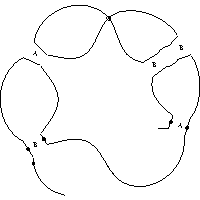
A doodle, or virtual doodle, flat knot or virtual flat knot or link may be described by a labelled peer code by designating the the appropriate crossing labels as flat, using the # character. Any virtual crossings are indicated using the * character. The following is an example of a doodle described by a labelled peer code:
[-15 -5, -1 -9 11, -13 7 -3]/# # # # # # # #
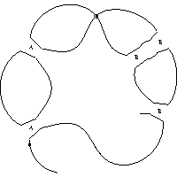
If we want a virtual doodle, or a virtual flat diagram, simply specify which crossings are virtual using the crossing labels.
[-15 -5, -1 -9 11, -13 7 -3]/# * * # # # # *
The draw programme converts input data in the form of a Gauss code to a labelled peer code and draws the diagram corresponding to the peer code. The conversion process is based on the algorithm used by Dror Bar-Natan and Jeremy Green in the production of their table of virtual knots. The user has no control over any virtual crossings that may need to be added during the conversion, they are determined automatically by the algorithm and, although some optimizations have been added to the original algorithm, virtual crossings are not guaranteed to be optimally placed in the immersion in every case.
To describe a diagram using a standard Gauss code, the classical crossings of the diagram are numbered arbitrarily and a code produced by following each component of the link from some arbitrary starting point, according to a chosen orientation. If a crossing is passed on an under-arc the crossing is written as a negative number and if the crossing is passed on an over-arc, it is written as a positive number. Multiple components are written separated by commas.
To indicate the nature of each crossing, as a positive or negative crossing, we append the sign of the crossing to the Gauss code following a '/' character. Thus an example Gauss code for a classical link is as follows:
1 -2 5 -4 3 -5, -1 2 -3 4 / ++--+
Note that the sign used in Gauss codes is the standard notion of a positive or negative crossing in classical knot theory. This is not the same as the use of signs in labelled peer codes.
Alternatively, Gauss codes may be specified as a sequence of terms of the form (O|U)<crossing-num><crossing-sign>, e.g. O1-O2+U1-O3+O4+U2+U3+U4+
The same under and over format may be used for virtual links by separating the crossing terms belonging to each component with a comma. An example of the Gauss code for a virtual link using the under and over format is U1+U2-,O3-,O1+O2-U3-.
Gauss codes may also be used to draw knotoids, or multi-knotoids. The Gauss code must describe the segment component of a knotoid first and must start at the leg of the knotoid. Moreover, in order to tell the programme that the Gauss code should be treated as a knotoid and not a virtual knot, the code must be preceded by "K:". An example of a multi-knotoid with four components described by a Gauss code is:
K:1 -2 10 -12, 4 -5 6 -7 8 -1 -3, 5 -8 2 3 -4, -13 9 -10 -11 14, -14 11 12 -9 7 -6 13 / - + + + + + + + - - - - - -
Multi-linkoids are described by Gauss codes by requiring that the open components are listed first and by indicating the number of open segments in parentheses, as in the following example:
K(2):7 -8 5,-2 3, 1 -3 4 -7 6 -5 -1 2 -4 -6 8/+ - + - + + - -

Here, there are two open components, one whose leg is the ingress over-arc at crossing 7 and whose head is the egress over-arc at crossing 5. The other open segment leg is the ingress under arc at crossing 2 and the head is the egress over arc at crossing 3.
The draw programme automatically converts muti-linkoid Gauss codes into labelled peer codes and draws then draws the corresponding immersion. The intermediate labelled peer code is recorded in the output file as part of the comment section before the metapost code for the diagram.
Diagrammatically, doodles, flat knots and their virtual counterparts are the same. As with classical or virtual diagrams, to create a Gauss code we number the flat crossings arbitrarily and assign an orientation to each component. Then, respecting that choice we trace the diagram following each component from an arbitrary staring point, noting the flat crossings encountered sequentially.
Two conventions are supported for specifying the crossing that we encounter as we trace the components. Following [3], since doodles and flat knots have no over of under crossings, we record whether the other strand crosses our path from left to right or from right to left, according to the given orientation. Crossing types are then labelled with the "flat" # decoration.
An example of a Gauss code for a doodle is:
L1 L2 R1 R2 L3 L4 R3 R4 / # # # #
The # labels may seem unnecessary but it allows common code for classical, flat, virtual and flat-virtual diagrams. Moreover, there is precedent for tautology within Gauss code syntax in the (O|U)-format above, where the sign of each crossing is specified twice. It therefore seems an acceptable demand that the crossing types are specified explicitly
The second convention supports the (O|U)-format Gauss codes used by J. Chen's FlatKnotInfo for specifying flat virtuals. Here the "O" is a synomym for "R", or "from the right" and "U" a synomym for "L", or "from the left", as in the first syntax. The difference is that the flat nature of the crossing is assumed, since the Gauss code does not describe virtual crossings. Thus an example Gauss code is simply:
O1O2O3U1U3U2
Internally, the draw programme converts this to the first format
R1 R2 R3 L1 L3 L2/# # #
In both cases the Gauss code is converted automatically to a labelled peer code from which the immersion is drawn. The intermediate peer code is recorded in the metapost output file. Here is an example drawn from the input code
O1O2O3O4O5U1O6U4U6U3U5U2

Diagrams with multiple components may be specified with either format, separating the crossing encountered on each component with a comma. Both of the following example Gauss codes will produce the same output
L1 L2 L3 R4 R5, L4 R6 R7 R1, L6 R8 R2 L9, L8 R3 R9 L5 L7/# # # # # # # # #
U1 U2 U3 O4 O5, U4 O6 O7 O1, U6 O8 O2 U9, U8 O3 O9 U5 U7
The draw programme supports planar diagram descriptions of knots, links, knotoids and multi-knotoids. Currently planar diagrams are assumed to describe diagrams involving classical crossings only, there is no support for flat crossings and therefore no support for doodles. Virtual knots and links are supported, as the programme treats planar diagram descriptions as an alternative description of a Gauss code. A planar diagram code is first converted to a Gauss code which is then converted to a labelled peer code.
To produce a planar diagram description of a knot, link or knotoid, the arcs between classical crossings (or the leg and head of a knotoid) are labelled sequentially from 1 as we trace each unicursal component. For virtual knots and links, the components may be considered in any order and with any chosen orientation and any arc may be chosen as the starting point for each component. There are additional requirements for knotoids, described below.
Having numbered a diagram, each crossing is described by the set of labels that appear at the crossing, using the standard convention of starting at the ingress under-arc and working anticlockwise around the crossing. The programme uses standard syntax to describe these labels; an example of the planar diagram description supported by the programme is:
X[3,1,4,2] X[4,2,5,3] X[7,6,8,5] X[6,1,7,8]
Spaces are permitted within the description and longer planar diagram descriptions may be broken across multiple lines of an input file using the escape character \ thus:
X[3,1,4,2] X[4,2,5,3] X[7,6,8,5] X[6,1,7,8]\
X[3,7,4,6] X[15,5,16,4]\
X[5,17,6,16], X[7,14,8,15] X[8,18,9,17] X[11,18,12,19] X[19,12,20,13], X[13,20,14,1]
Knotoids may be described by planar diagrams by preceding the description with "K:", as in the case of Gauss codes. For knotoids and multi-knotoids, it is required that the numbering start at the leg of the segment component of the knotoid, so that the arc containing the leg is numbered 1. It is also required that the description of the crossing involving the leg of the knotoid appear first in the list of crossings. The following is an example of a knotoid described by a planar diagram:
K:X[4,1,5,2] X[2,6,3,7] X[7,3,8,4] X[5,8,6,9] X[9,11,10,12] X[10,12,11,1]
Note, planar diagrams are not suitable for describing multi-linkoids, since they contain no implicit ordering of components, so it is not possible to specify which are to be regarded as open and which closed.
The command syntax for the programme draw is as follows:
draw [--<programme-option>][-<metapost-control>][<infile>[<outfile>]]
The programme reads labelled peer codes from the <infile>, or from a command prompt if no <infile> is provided, and then evaluates a triangulation of the disc determined by the immersion underlying the peer code.
By default, the programme uses Ken Stephenson's circle packing algorithm to place the vertices of the triangulation. Alternatively a <programme-option>, as described below, may be used to select a different vertex placement technique.
Once the vertices have been positioned, the programme creates a metapost script describing the diagram in <outfile>, or in the file draw.out if no <outfile> is provided.
The supported programme-option and metapost-control options are:
<programme-option>
  convex-disc: draw the convex, straight line triangulation of a disc
  edge[=<max-iterations>] default 200: use edge distribution placement
  force[=<max-iterations>] default 200: use Plestenjak force directed placement
  gravity[=<max-iterations>] default 200: use centre of gravity placement
  hamiltonians: draw all Hamiltonian circuits for a given diagram
  hamiltonian_circuit[=e_1 ... e_n]: draw a single Hamiltonian edge circuit for a given diagram
                                     if no explicit edge circuit is given, draw any Hamiltonian circuit
  laces: draw lace diagrams from the programme input
  magnify[=<percentage>] default 0: magnify small circles in circle packing by specified percentage
  seifert-circles: draw the Seifert circles determined by the label orientation of the given diagram
  shrink[=<max-iterations>] default 200: use region shrinking placement after circle packing
  small-shrink[=<max-iterations>]: use small region shrinking placement after circle packing
  smoothed: draw all of the smoothed states for the given diagram

<metapost-control>
  c=<centre>: specify the centre of rotation <centre> = (<x>,<y>)|z<n>
  C=<cycle>: specify the turning cycle to bound the infinite region
  D: set the smoothed state disc size multiplier to determine the size of smoothed crossings n*d (default n=6)
  d: set the unit multiplier to determine the crossing disc diameter (default 30)
  F: do not draw the crossing features
  h: help screen
  I: do not draw the immersion (consider using F option also)
  k: draw knotoids with the leg in the unbounded component of the immersion's complement
  l: add edge labels to the diagram
  o: draw orientation for knots (orientation always shown for knotoids)
  p: set the pen multiplier n to determine the pencircle scale n*0.5pt (default n=1)
  P: draw the underlying circle packing that determines the diagram
  r=<degrees>: rotate the diagram anti-clockwise by the specified number of degrees
  S: draw the shortcut if the code describes a knotoid
  t: draw the triangulation of the unit disc
  u: set the unit dimension nn to determine u=0.nn points (default 20)
  v: label the vertices and draw coordinate axes
The short <metapost-control> options have corresponding long options, useful for including in input files as global options or as qualifiers (see the section Input file format):
  centre=<centre>: specify the centre of rotation <centre> = (<x>,<y>)|z<n>
  cycle=<cycle>: specify the turning cycle to bound the infinite region
  dots: draw knotoid shortcuts dashed with dots rather than dashed evenly
  disc-size: set the unit multiplier to determine the crossing disc diameter (default 30)
  knotoid-leg-unbounded: draw knotoids with the leg in the unbounded component of the immersion's complement
  labels: add immersion edge labels to the diagram: by default immersion edge labels are numbered from 0 (see the L option)
  no-crossings: do not draw the crossing features
  no-immersion: do not draw the immersion
  oriented: draw orientation for knots (orientation always shown for knotoids)
  packing: draw the underlying circle packing that determines the diagram
  pen-size: set the pen multiplier n to determine the pencircle scale n*0.5pt (default n=1)
  rotate=<degrees>: rotate the diagram anti-clockwise by the specified number of degrees
  shortcut: draw the shortcut if the code describes a knotoid
  triangulation: draw the triangulation of the unit disc
  unit: set the unit dimension nn to determine u=0.nn points (default 20)
  vertices: label the vertices and draw coordinate axes
additional long options:
  colour: draw different components with colours rather than just black lines
  colour-map=<filename>: use the colours in <filename> rather than the default colours
  cusp_disc_size=<n>: set the cusp disc size multiplier to determine the size of the non-Seifert-smoothed cusp indicator discs, n/10*disc-size (default n=7)
  edge-factor=<float> default 0.5: amount by which vertices are moved towards the COG in edge distribution placement
  first-gap: always use the first gap as the active gap in edge distribution placement
  frame-corners: show frame corners when tracking placement iteration
  gauss-crossings: show labels for the Gauss crossings, as specified by Gauss code or planar diagram input, or calculated from peer code input
  gauss-labels: show labels for Gauss arcs, not immersion arcs: gauss-labels are numbered from 1
  grid[=<grid-size>]: draw a grid to assist with using the translate option (default 10)
  hyperbolic: drawing diagram in the hyperbolic plane
  label-shift=<n>: set the number of units u by which the labels of small smoothed crossings should be moved (default n=50)
  no-vertex-axes: do not show the axes when labelling the vertices of a diagram
  no-show-displacement: do not show the triangulation displacement when tracking placement iteration
  odd-parity-disc-size=<n>: set the odd parity disc size multiplier to determine the size of the odd parity crossing indicator, n/10*disc-size (default n=12)
  parity: show crossings with odd parity in smoothed states
  plot[=<divisions>]: set the number of divisions for the histogram in edge distribution placement (default 20)
  scale=<float>: override other size settings and scale diagram to the specified multiple of a standard size
  script-labels: label vertices using TeX's script size font
  scriptscript-labels: label vertices using TeX's scriptscript size font
  seifert-edges: highlight the odd or even immersion edges, so edges belonging to the same Seifert circle have the same colour
  show-shrink: draw the effect of shrinking the triangulation when using region shrinking placement
  show-small: highlight the small edges of the triangulation when using edge_distribution placement
  shrink-factor=<float> default 0.75: amount by which region shrinking placement retracts trianglulation
                                         vertices towards the barycentre
  shrink-area-factor=<float> default 1.618034: region shrinking placement converges if all compact
                                               regions have an area within this factor of their average area
  smoothed-disc-size: set the smoothed state disc size multiplier to determine the size of smoothed
                      crossings n*disc-size (default n=6)
  smoothed-disc-threshold=<n>: set the diameter in units u of the smoothed crossing disc below which the label of the crossings should be moved (default n=30)
  state: specify the smoothed state that you wish to draw as a string of A and B characters corresponding to the Gauss crossings of the diagram
  tranlsate=<translation-list>: specify a list of vertices together with a translation in the form UxPyR:VxQyS... where U and V
                               are vertex numbers and P,Q,R,S percentages of the diagram width and height e.g. 10x8y-33 indicates
                               shifting vertex 10 +8% to the right -3% up
  tension: set the metapost path tension, default value 1.0, i.e. the metapost ".." default
  uniform-smoothed-discs: always draw state smoothed discs of the size specified by smoothed-disc-size
additional short options:
  #: debug
  a=<float> default 1.0: average triangulation edge length factor
     used to magnify edge vertices closer than a*average_triangulation_edge_length
  A: adjust the angle of diagram arcs at crossings to be right angles
  b: do not use badness optimization
  B: include boundary vertices; may be used with f, g, P, or t.
     Boundary vertices are alway included in force directed placement,
     in which case this option only has an efect if the t option is also used.
  E: use edge repulsion rather than Plestenjak force directed placement
  i[=<max-iterations>] default 1000: set maximum circle packing iterations
  H!: additional help screen
  #H!: display debug help screen
  K: use Fenn's circle packing algorithm rather than Ken Stephenson's
  L: start from one when labelling edges
  M=<scale_factor> : set metapost_coordinate_scale_factor: default 2500 with the circle packing
     option, 1000 with force or gravity placement, 600 with the convex-disc option, 25 otherwise
  O: turn off default one_metapost_path and use two paths for each component with explicit direction, rather than a cycle
  P: draw circle packing
  R=<float>: retract boundary vertices radially towards their centroid by a factor <float> < 1
  T[=<track-step>] default 1: track placement iteration (force, gravity, shrink)
  V[=<vertex>] default 0: check inner hull calculation of <vertex>
The overlap between long options and short options is designed to provide a convenient mechanism for setting programme defaults from the command line as well as an intuitive approach to creating input files (see below)
By default the draw programme produces metapost code based on the following metapost parameters
The metapost code produced by the programme expresses dimensions as multiples of a unit parameter, u, whose default value is shown above. The overall size of a diagram may therefore be modified by adjusting the unit size.
For large diagrams, metapost can sometimes complain that a quantity is too large, in which case reducing the unit size will typically solve the problem. If the diagram coordinates are still too large, the metapost_coordinate_scale_factor may be adjusted using the M option. This scale factor is dependent on the drawing algorithm and is used to adjust coordinate values produced by the algorithm so they are more readily handled by metapost.
There is also a scale=<float> option that adjusts the size of a diagram so that the range of x and y coordinates determine a rectangle whose diagonal is the given floating point multiple of 100 pts (about 35mm). The scale option was added so that an input file that would normally produce different sized diagrams may be scaled automatically so that all the diagrams are roughly the same size. This is particularly useful for displaying several diagrams in a paper or on a website.
To represent crossings, the metpost code places a disc at a crossing vertex and then draws an over-arc, or creates a virtual crossing glyph as required by the diagram. The size of these disc is controlled by the disc-size (or the short d) option. As can be seen from the default value shown above, increasing the unit size also increases the disc size, so it is sometimes useful to control the two quantities separately.
The pen-size determines the thickness of the lines in the resulting diagram, by controlling the size of pencircle used by metapost.
The section Example diagrams below provides a description and some examples of the most common drawing options.
Multiple peer codes, Gauss codes, or planar diagrams may be included in an inputfile, one per line. As mentioned above for planar diagrams, long input strings may be broken across multiple lines by including an escape character \ at the end of a line. Note, however, that for peer codes and gauss codes you cannot use an escape character after the / character within the code.
Default options to be applied to all the codes in the file may be specified from the command line using long or short options. Alternatively, defaults may be included within the file itself by specifying one or more long options within square brackets, separated by commas, as in [unit=30,labels]. It is possible to override the defaults on a per-code basis by including qualifiers after a peer code. Qualifiers are long options, separated by commas, included within braces {}
The input file may contain comments by inserting the ; character anywhere on a line. Any text on a line following a ; is ignored.
Input codes in a file may be provided with a title that is reported in the output of the programme. Titles are specified by starting a line with --.
You can force the programme to stop processing input codes in an input file at any point by including the word exit at the start of a line.
An example input file is:
; here is an example input file

[oriented, unit=30] ; set default options for all of the codes in this file

-- an example of a flat knot; this is a comment on a title line
[-5 -7 -1 -9 -3]/#####

-- a rotated knotoid
[-7 13 -11 -1 3 -5 9^ ]/+ + - + + - - {rotated=45, centre=z4}

; un-commenting the following line causes the programme to stop reading the input file at this point
; exit

; here is the Gauss code of a knot in OU format with an instruction to use cycle 6 as
; the infinite turning cycle (see Example diagrams below))
O1+O2+O3+U1+O4-U2+U4-U3+{cycle=6}

; here is the standard Gauss code of a link
-1 3 5 6, 2 -3 4 -6, 1 -4 -5 -2/+ - - + + +
In the above example a diagram is rotated by 45 degrees about z4. The default centre of rotation is determined from the minumum and maximum x-coordinates and y-coordinades, the midpoint of each being used to determine the centre of rotation. In the above example an explicit centre of rotation is given as one of the vertices used to draw the diagram. The metapost path created for each diagram has a vertex at each crossing and a vertex at the midpoint of each semi-arc. A diagram with the vertices labelled may be drawn using the long option vertices or the short option v (see below for an example). Alternatively, an explicit centre of rotation may be specified by giving the exact x and y coordinates.
Some examples of the diagrams that the programme can produce are shown below, these pictures are png format files generated by Ghostscript
The following is an example of the diagram resulting from the metapost code produced by the draw programme for the virtual knot [-5 7 9 -11 3 1 ]/+ + * + + +

[-7 39 -53 27 15 35 -47, 13 -43 37 -45, 49 -33 -21 -41 5 19 11 -23 -51 -29 1, -31 25 -9 -17 -3]/- + - + - + + - + + + + + + + - - - - + - - + - - + -

Using the --oriented/-o option adds the orientation determined by the immersion code:

Using the --label/-l option produces labels on the edges of the diagram. By default the programme labels each semi-arc of the immersion, meaning that each semi-arc either side of a virtual crossing is assigned a different label. If you want to label the arcs between classical crossings only, use the option --gauss-labels. The following is an example of the default labelling:

Using the --gauss-crossings option produces labels at the Gauss crossings of the diagram. That is, at the non-virtual crossings that are described by the the Gauss code that underlies the diagram. If the diagram was constructed from a Gauss code or planar diagram input, the Gauss crossings correspond to those described by the input code. If the diagram was constructed from a labelled peer code, the numbering of the Gauss crossings is determined by the order in which the crossings are first encountered when tracing the diagram in a manner determined by the edge labels of the peer code, as can be seen in the following diagram by comparison with the label example above:

You can instruct the programme to use TeX's mathematics "script size" or "scriptscript size" font for semi-arc or crossing labels with the script-labels and scriptscript-labels options respectively.
Using the --vertices/-v option produces a diagram with coordinate axes and vertex labels, intended to aid the case where the Metapost code requires manual adjustment:

The following is an example of the diagram resulting from the metapost code produced by the draw programme for the knotoid
[-7 13 -11 -1 3 -5 9^ ]/+ + - + + - -

If the --knotoid/-k option is used the leg appears in the unbounded component of the knotoid complement, however, as in the following example this does not always produce an aesthetic result.

If the --shortcut/-s option is used the shortcut is drawn:

% -- Example immersion
% [4 8 0 2 6]/# # # # #
% left turning cycles:
% cycle 0: 0 6
% cycle 1: -1 -5
% cycle 2: 2 8 4
% cycle 3: -3 -7 -9
% right turning cycles:
% cycle 4: 0 -5 2 -7
% cycle 5: -1 6 -9 4
% cycle 6: -3 8
% infinite turning cycle = 4
See labelled-peer-code.pdf for an explanation of the minus signs in this output.
From this information it is possible to select a particular turning cycle if required. For example, the peer code[5 7 1 9 3]/##### {labels}
produces the following immersion diagram
and the turning cycle information shown above. If we select cycle 2 and use the qualifier:
[5 7 1 9 3]/##### {labels,cycle=2}
we produce the following diagram.

Note: sometimes the Metapost code produced by the draw programme results in Metapost producing postscript files with negative bounding box values. For some programmes it is therefore necessary to add the following line to these postscript files
<x-shift> <y-shift> translate
where <x-shift> and <y-shift> are chosen so the lower-left bounding box coordinates are non-negative.
By default the draw programme produces black and white diagrams but it is possible to create coloured drawings using the command line options colour and colour-map. The programme makes use of the metapost mpcolornames package and can draw an entire diagram with a different colour using the option colour=<colourname>, or it can draw each component of the diagram with a different colour by using the option colour without specifying a particular colour. By default, this results in the components being coloured in the order "red","blue","ForestGreen","Brown","DarkViolet",and "Orange". Any subsequent components are drawn black.
Additional colours, the colour selection, or the order in which colours are used may be changed by using the colour-map=<colour-map> option, which takes a colour-map file name as a parameter, see section Draw programme command syntax below. A colour-map file is just a list of the colours to be used in order, one per line. If there are more diagram components that there are colours specified in the colour-map file, then subsequent components are drawn black.
Any valid mpcolornames colour may be specified in a colour-map file.
In some cases, despite the range of options provided by the programme, the circle packing, or alternative, drawing algorithm may cannot arrange the vertices used to draw a diagram in an aesthetic manner and it is necessary to adjust their position manually. To support this, the programme provides a translate option that allows vertices to be moved relative to the overall size of the diagram.
As shown above in the section Example digrams, the vertices option displays the coordinate axes and the maximum and minimum coordinate values of the vertices used to draw the underlying immersion diagram. The translate option allows vertices to be moved by a percentage of the difference between these minimum and maximum values with respect to the coordinate axes. Thus, in the example shown below, the minimum and maximum x-coordinates are -1091 and 175 units, so we can move vertices in steps of (175-(-1091)/100 = 12 units (using integral division) in the x-direction. Similarly, the minimum and maximum y-coordinates are -723 and 250 units, so we can move vertices in steps of 9 units in the y-direction.
The syntax for specifying the required translation is translate=UxPyR:VxQyS:... where U and V are vertex numbers, P and Q are the number of steps in the x-direction and R and S are the number of steps in the y-direction. Thus, the option translate=0x5y7:2x-3y4:10x7y-4 move vertex z0 5 steps in the x-direction and 7 in the y-direction, moves z2 -3 steps in the x-direction and 4 in the y-direction and moves z10 7 steps in the x-direction and -4 in the y-direction.
In most cases the translate option is most usefuly added as an qualifier to an input code within an input file.
The grid option may also be used to draw a grid based on the minimum and maximum coordinate values to assist with the use of the translate option. By default the grid size is ten percent of the difference between the maximum and minimum coordinates of the corresponding dimension. If required, the grid size may be set by appending a value to the option: grid=<grid-size>, specifying the desired percentage.

There are several invariants based on state sums for which it is sometimes useful to generate pictures of the smoothed states for an example diagram. By using the smoothed programme option, the draw programme will produce metapost code for all of the smoothed states of each input code.
Only non-virtual crossings are smoothed, and in the case of knotoids, shortcut crossings are not smoothed. For the remaining crossings, the states range over all combinations of Seifert-smoothed and non-Seifert-smoothed choices for each crossing. A Seifert smoothed crossing is one for which the smoothed state corresponds to tracing the Seifert circles of the underlying diagram at that crossing.
The smoothed option produces a diagram of the original knot or knotoid, with semi-arcs labelled from zero as determined by the labelled peer code. Then it produces state diagrams, identifying each non-Seifert-smoothed crossing by marking the crossing cusp with a small black dot on each smoothed strand. The size of this dot may be controlled by the option cusp-disc-size, see the section draw programme command syntax for details.
Each smoothed crossing is labelled with its state as follows:
The size of a smoothed crossing is governed by the long option smoothed-disc-size or corresponding short option D, which defaults to six times the size of a un-smoothed crossing disc. If the arcs involved in a smoothed crossings are positioned in such a way that the current value of this option is too large for the smoothed crossing to be drawn correctly, the programme will automatically reduce the size of the smoothed crossing disc to an appropriate size, unless the option uniform-smoothed-discs has also been used. This is because, in some cases, reducing the size of the smoothed crossing using the smoothed-disc-size option, or additionally adjusting the crossing disc size with the disc-size or d may be preferable.
If a smoothed crossing is small it may be the case that the default approach of labelling smoothed crossings at the centre (the location of the intersection in the underlying immersion) makes the labels difficult to read, even if they are adjusted using the script-labels or scriptscript-labels option. In this case the labels are moved to one side of the crossing by an amount controlled by the label-shift option, which defaults to 50 units. The option smoothed_disc_threshold, which defaults to 30 units, determines the threshold for the diameter of a smoothed crossing disc below which the label is moved to the side.
The following is an example of a smoothed state for a knotoid that closes to the Slavik knot:


The full set of smoothed states for this knotoid are as follows:


In some cases it is useful to identify which crossings have odd Gaussian parity, as described in [2]; that is, appear in a Gauss code with an odd number of terms between the two occurrences of the crossing, or equivalently, are represented on a Gauss diagram by a chord that is linked with an odd number of other chords.
The draw programme provides a parity option that causes the programme to replace odd crossings with a graphical node. The parity option may be used by itself or in conjunction with the smoothed option, in which programme draws all of the states corresponding to smoothing the even crossings. The option may also be used with the state option as described below.
The option odd-parity-disc-size may be used to control the diameter of the graphical node used to represent odd parity crossings. See the section draw programme command syntax.
You can draw an individual smoothed state using the state=<state-string> option, where the <state-string> is a sequence of A and B characters identifying whether a crossing should be A-smoothed or B-smoothed.
Crossing designations as either A or B are required for each crossing in a diagram that is smoothed. Thus, for Gauss code input and planar diagram input a designation is required for each crossing and for peer code input a designation is required for each non-virtual and non-shortcut crossing.
The crossing designations are specified in ascending order corresponding to the crossing numbering used by the type of input provided. Thus, when used with a Gauss code, the crossing numbering is that used by the Gauss code. When used with a labelled peer code the crossing numbering is that determined by the naming edges of the peer code and when used with a planar diagram the crossing numbering is determined by the order in which the crossing data is provided.
If the parity option is used at the same time as the state option, state designations are required only for the even crossings and are, again, specified in ascending order corresponding to the crossing numbering determined by the input format provided. In the first of the following examples, without the parity option, a state designation is required for all six crossings, whereas in the second example only two designations are required since only the first and fourth crossings are even.
X[4,1,5,2] X[2,6,3,7] X[7,3,8,4] X[5,8,6,9] X[9,11,10,12] X[10,12,11,1] {state=ABABAB}
X[4,1,5,2] X[2,6,3,7] X[7,3,8,4] X[5,8,6,9] X[9,11,10,12] X[10,12,11,1] {state=AB,parity}
To identify the even crossings it can be helpful to draw the diagram using the gauss-labels option. The left hand diagram below was generated using the input:
X[4,1,5,2] X[2,6,3,7] X[7,3,8,4] X[5,8,6,9] X[9,11,10,12] X[10,12,11,1] {parity,gauss-labels}
the right hand image was generated using the options {state=AB,parity}, as shown above.


I am grateful to Maciej Borodzik for suggesting adding the capability to draw a single state.
A common smoothed state for a diagram is where each crossing is Seifert-smoothed to yield a set of Seifert circles for the diagram. This smoothed state is supported directly with the seifert-circles option. Using this option draws only the Seifert circles, not any of the smoothed crossing state information.
When drawing Seifert circles, the smoothed-disc-size and uniform-smoothed-disc options can be useful to produce more aesthetic diagrams. For example:


Here, the middle diagram was drawn using the default options and the right hand diagram used --uniform-smoothed-discs --smoothed-disc-size=3 .
Note that whilst smoothed states A and B are only defined for classical crossings, Seifert circles are supported for flat crossings as well, so the programme can draw Seifert circles for doodle diagrams.
There is also a seifert-edges[=odd] option that highlights the edges of a diagram that belong to the same Seifert circle using colour. By default, the option causes the edges with an even immersion label to be drawin in red and those with an odd immersion label drawn in black. This results in a diagram with red and black Seifert circles. If required, the optional =odd option may be given, which draws the odd labelled edges in red and the even edges in black.
The draw programme has the ability to look for Hamiltonian circuits in a diagram involving only classical or flat crossings. It can draw every Hamiltonian circuit, or just the first Hamiltonian it finds, or you can draw a specific circuit, specified as a sequence of edge labels (see the --labels option above). The hamiltonians option produces a set of all possible Hamiltonian circuits, whereas the hamiltonian-circuit option produces a single diagram of the first Hamiltonian found by the search algorithm. If you specify a sequence of edge labels as in hamiltonian-circuit=0 5 10 9 3 2 7 12 , then the programme draws the given circuit.
By default, the programme highlights the Hamiltonian circuit in green, as in the following diagram

You can control the colour used for the Hamiltonian circuit using the hamiltonian-colour option, which can be used in conjunction with the colour options described in the section Adding colour. For example, the following diagram was produced using the options --colour --hamiltonian-colour=black.

Version 1: support for Knotoids; identified by extending peer codes and immersion codes to allow a '^' character following a crossing number to indicate the first shortcut crossing.
Version 2: added immersions and rotation.
Version 3: added labelled peer codes and Metapost control qualifiers.
Version 4: added drawing of the triangulation underlying the circle packing.
Version 5: added Fruchterman and Reingold force directed placement added edge magnification.
Version 6: added inner hull and centre of gravity.
Version 7: ported Ken Stephenson's circle packing algorithm to C++ and added check for connected code data.
Version 8: replaced Fruchterman and Reingold force directed placement with the Plestenjak modifications updated the triangulation for diagrams having two edges in the infinite turning cycle.
Version 9 (December 2017) Added capability to draw straight-edge disc triangulations from either peer-code triangulations or dedicated input files.
Version 10: reinstated a form of Fruchterman and Reingold force directed placement where adjacent type 1 and type 2 vertices that are too close to each other repel.
Version 11 (October 2018)) added region shrinking placement, rearranged and improved the use of long and short programme options.
Version 12: added the ability to the draw smoothed states for a given knot, link knotoid or multi-knotoid diagram.
Version 13: (December 2021) added lace drawing capability, the ability to draw diagrams with colour and support for diagrams containing Reidemeister I loops.
Version 14 (December 2021) added the ability to draw knots from Gauss codes and added the smallarrowheads option.
Version 15 (January 2022) added the ability to label Gauss-arcs rather than immersion edges.
Version 16 (February 2022) added the ability to draw a single smoothed state rather than all of them.
Version 17 (March 2022) added planar diagram support and optimized the Gauss to peer code conversion.
Version 17.1 (March 2022) added automatic sizing of smoothed crossings and the ability to shift smoothed crossings labels to one side.
Version 18 (October 2022) added labelling of Gauss crossings, as specified by Gauss code or planar diagram input, or calculated from peer code input.
Version 19 (August 2023) added the ability to draw multi-linkoids, added shorcuts to knot-type knoid drawings, added the scale option to re-size diagrams so they become proportional to a fixed diagonal size
Version 20 (October 2023) added the ability to draw Seifert circles and Hamiltonian circuits
Version 21: (November 2023) improved the drawing of multi-linkoids, updated and made default the use of a single metapost path per component added seifert-edges option
Version 22: (November 2024) added support for the Gauss code format used by J. Chen's FlatKnotInfo
Version 23: (December 2024) changed the syntax for multi-linkoids to use '%' for knot-type components. Introuduced support for singular crossings using the label '@'
Version 23.1: (February 2026) Code update and bug fixes
[1] Knotoids, Vladimir Turaev, arXiv:1002.4133v4.
[2] Parity in knot theory, (Russian), V. O. Manturov. Mat. Sb., 201, (2010), no.5, 65-110; translation in Sb. Math., 201, (2010), no. 5, 693-733
[3] A. Bartholomew, R. Fenn, N. Kamada, S. Kamada, On Gauss codes of virtual doodles (Journal of Knot Theory and Its Ramifications Vol. 27, No. 11, 1843013 (2018), arXiv:1806.05885).